AIoT LABORATORY / UBICOMP & ISWC 2026
Building Reproducible
Wi-Fi RF Fingerprinting Pipelines
Signal Collection, Datasets, and Evaluation
Follow the lecture, work through three labs, and build a Wi-Fi device-identification pipeline with SMoRFFI.
123 same-model IoT devices · Prepared Wi-Fi records · Laptop-based labs
OVERVIEW
What this tutorial covers
This tutorial teaches a reproducible Wi-Fi radio frequency fingerprinting (RFF) workflow for IoT device identification. Participants follow the complete path from Wi-Fi signal acquisition concepts to dataset inspection, RF feature construction, baseline identification, error analysis, and reproducible reporting.
The hands-on part uses prepared Wi-Fi RFF records, extracted RF features, executable notebooks, and reference outputs. Participants can complete the labs with a laptop. The instructors will demonstrate the acquisition workflow with SDR hardware and GNU Radio, while the executable labs use prepared data to keep the session stable.
The tutorial is built around the SMoRFFI dataset and framework. SMoRFFI was collected from 123 same-model commercial IEEE 802.11g IoT devices and contains 35.42 million raw I/Q preamble samples with 1.85 million extracted RF features. The accompanying framework covers data collection, feature extraction, and benchmark evaluation.
Why this tutorial matters
RF fingerprinting uses transmitter-dependent hardware imperfections in radio signals for device identification. This physical-layer signal provides a useful complement to software-level identifiers such as MAC addresses, which can be changed, randomized, or reused.
Reproducible RFF experiments require several pieces of practical knowledge:
- Wi-Fi packet structure and preamble records;
- SDR-based collection and synchronization;
- signal preprocessing and feature construction;
- dataset organization and label checking;
- train-test split design and leakage control;
- baseline reproduction, debugging, and reporting.
Same-model device identification is a demanding learning setting. Devices share the same vendor and model, so easy model-level differences are removed. Participants need to examine feature behavior, confusion patterns, sample budgets, and evaluation choices.
End-to-end pipeline
The tutorial follows four pipeline stages.

| Stage | Main Question | Tutorial Output |
|---|---|---|
| 1. Wireless signal acquisition | How are Wi-Fi preamble records captured from transmitters? | Acquisition workflow steps and hardware walkthrough notes |
| 2. RF feature construction | Which features describe transmitter-dependent signal behavior? | Feature table, visualization, and quality checks |
| 3. Recognition and decision | How does a baseline model identify devices from RF features? | Trained classifier, prediction table, and metrics |
| 4. Evaluation and deployment | How should an RFF experiment be checked? | Accuracy, recall, F1-score, confusion matrix, and reproducibility checklist |
Each section follows the lecture slides. Use the arrows to turn pages, or open the chapter PDF. Run the notebook during Labs 1-3 and compare the outputs with the examples.
SESSION INFORMATION
Information and schedule
| Item | Information |
|---|---|
| Topic | Wi-Fi RF fingerprinting for IoT device identification |
| Tutorial style | Short lectures, guided notebooks, hardware walkthrough, debugging, and discussion |
| Target participants | Students, researchers, and practitioners in ubiquitous sensing, IoT systems, wireless sensing, edge intelligence, and physical-layer security |
| Hands-on requirement | Laptop and web browser (Github and Kaggle) |
| SDR experience | No prior SDR experience is required for the hands-on labs |
| Main data source | SMoRFFI Wi-Fi RFF records and extracted RF features |
| Expected outputs | Dataset overview and field list, feature visualizations, baseline model, accuracy report, confusion matrix, and reproducibility checklist |
| Local execution (optional) | Python 3.10 or later, Jupyter, NumPy, pandas, scikit-learn, matplotlib |
Session schedule
| Time | Module | Activity | Output |
|---|---|---|---|
| 15 min | Task Introduction | Define RF fingerprinting for IoT device identification and introduce the reproducibility problem. | Task definition and pipeline map |
| 25 min | Signal and Feature Introduction | Introduce Wi-Fi preamble records and the RF features used in the labs. | Feature reference sheet |
| 20 min | Data Acquisition Pipeline Walkthrough | Present the USRP B210, GNU Radio, Wi-Fi AP, and M5Stack collection workflow. | Acquisition workflow notes |
| 30 min | Lab 1: Load and Explore the Dataset | Compare the two dataset views, inspect labels, count records, and identify feature fields. | Understanding of the two dataset views and their fields |
| 20 min | Coffee Break and Hardware Display | Inspect the USRP B210, M5Stack transmitter, and acquisition setup materials. | Hardware Q&A |
| 30 min | Lab 2: Construct and Visualize RF Features | Compute or inspect selected RF features and visualize distributions across devices. | Feature plots |
| 30 min | Lab 3: Build and Evaluate the Baseline | Train the baseline classifier, generate predictions, and inspect accuracy and confusion patterns. | Metrics and confusion matrix |
| 20 min | Debug and Output Checking | Compare notebook outputs with reference outputs and resolve setup issues. | Passed checkpoints |
| 20 min | Wrap-up and Open Discussion | Discuss workflow adaptation, dataset scope, reproducible reporting, and open research problems. | Reproducibility checklist |
COURSE MATERIALS
Materials & practical information
Materials and links
Chapter PDFs are available inside each teaching section. Slides are supplied as PDF; the editable PowerPoint source can be added when available.
The dataset and notebook links above are the resources shown in the slides.
- Official UbiComp/ISWC 2026 Workshops and Tutorials page: https://www.ubicomp.org/ubicomp-iswc-2026/workshops-and-tutorials-2026/
- Current tutorial page: https://www.aiotlabs.org/ubicomp2026-rff-tutorial/
- Data Acquisition System: Dockerized-wifi-iq-preamble-capture
- SMoRFFI article DOI: 10.1016/j.comnet.2026.112309
GUIDED SESSION · 15 min · SLIDES 3-8
Background and Task Introduction
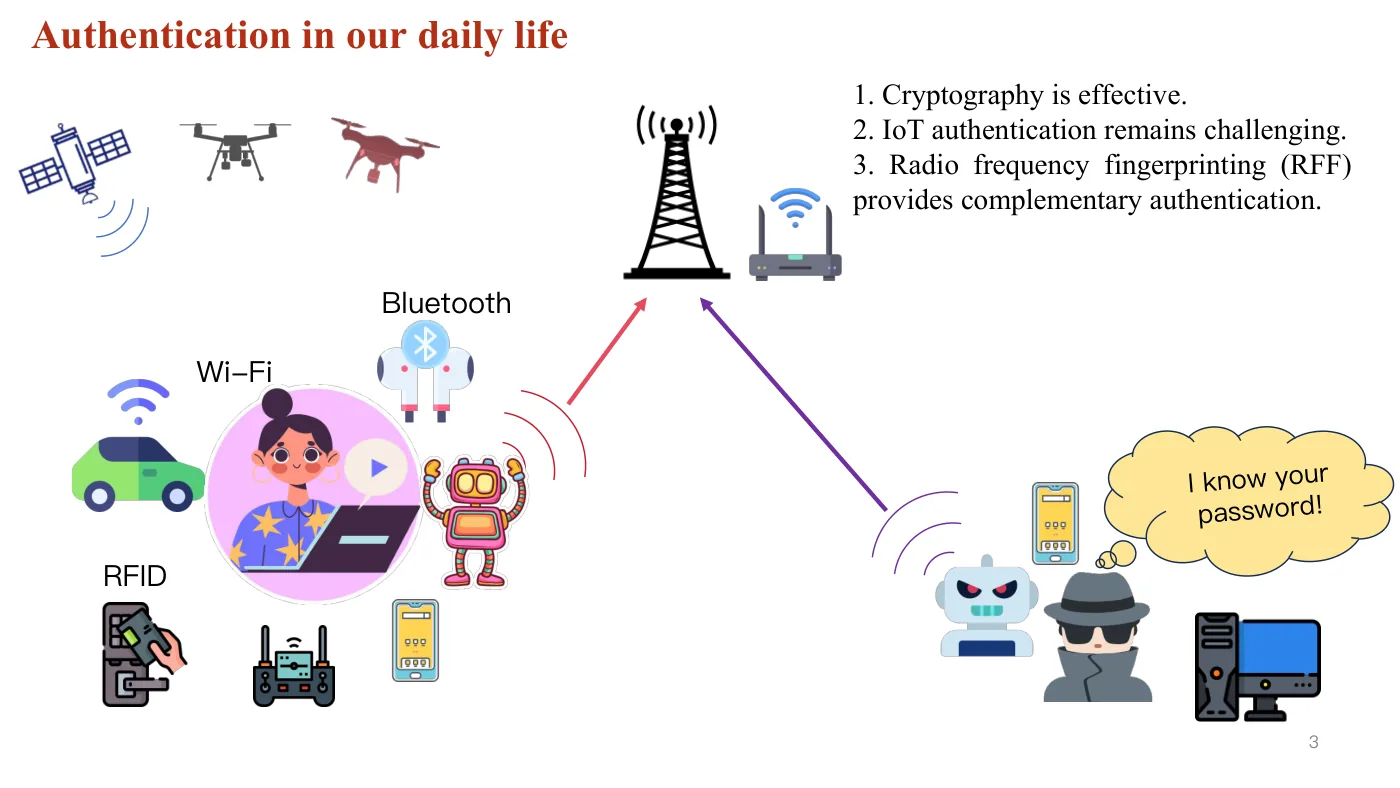
Identify a Wi-Fi transmitter from the RF features in its recorded signal.
Our task today
The slides introduce verification, identification, and device-type classification. Our hands-on task is device identification: the model predicts a device label from prepared Wi-Fi records.
Follow the same experiment from beginning to end: inspect the data, calculate RF features, and run a Random Forest baseline.
Learning objectives
By the end of the tutorial, participants will be able to:
- explain the Wi-Fi RFF acquisition process, including packet transmission, preamble capture, and record generation;
- load Wi-Fi preamble and RF feature records into a reproducible notebook workflow;
- inspect device labels, sample counts, feature fields, and basic data quality checks;
- compute or interpret selected RF features, including CFO, phase error, magnitude error, I/Q gain imbalance, and fractal dimension;
- visualize feature distributions and device-level separability;
- train a baseline device-identification model and report accuracy, recall, F1-score, and confusion patterns;
- compare intermediate outputs with reference results;
- adapt the workflow to a new wireless sensing or physical-layer identification dataset.
GUIDED SESSION · 25 min · SLIDES 10-20
Signal and Feature Introduction
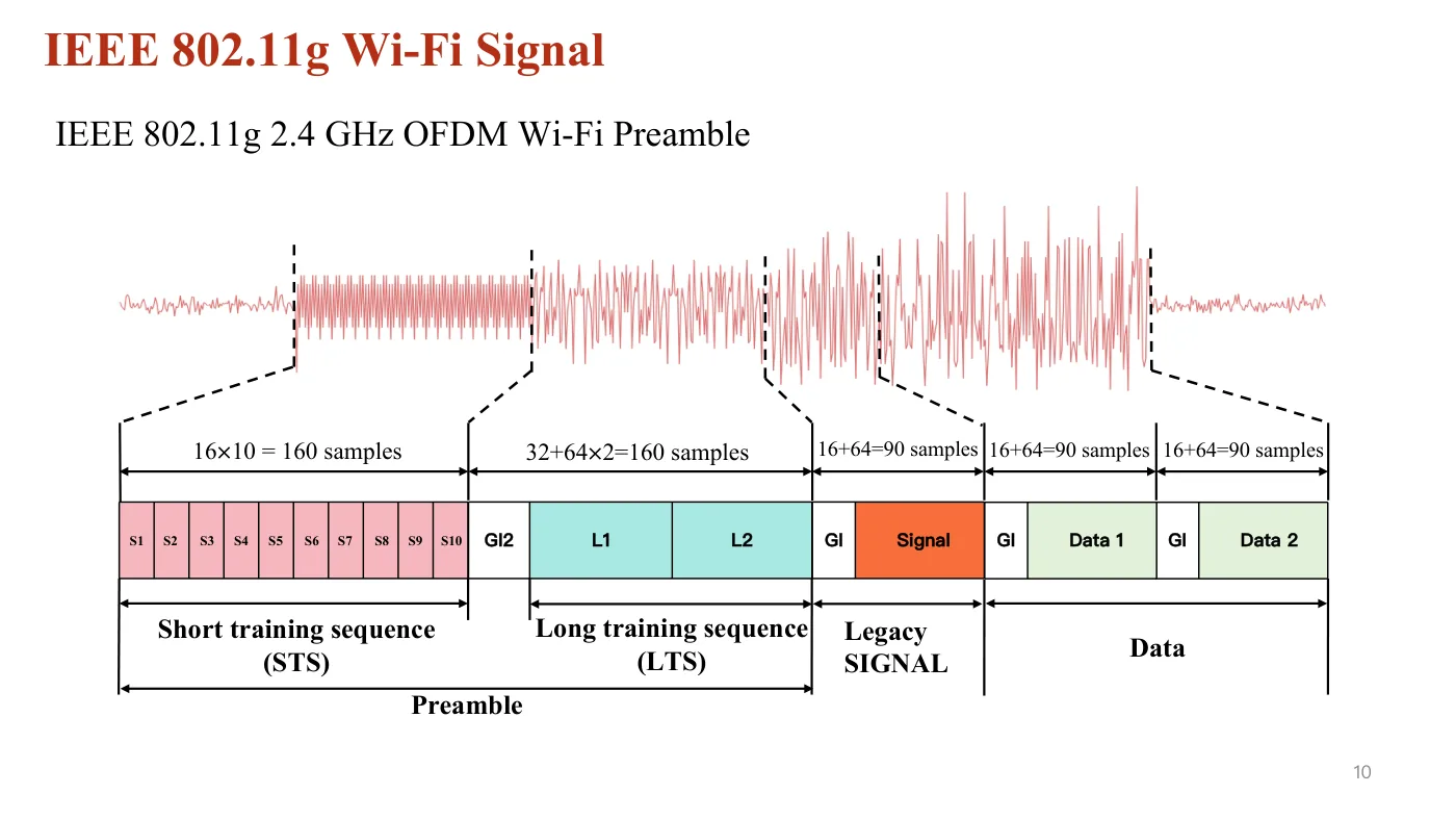
Connect the preamble in a Wi-Fi record to the features used in the labs.
Read the diagrams in order
Start with the Wi-Fi preamble on slide 10. Locate the short training sequence (STS) and long training sequence (LTS). Then follow the extraction diagram on slide 12.
Slides 13-19 introduce CFO, phase error, magnitude error, I/Q imbalance, and fractal dimension. For each feature, connect its meaning to the example plot.
Recognize the feature names and the signal stages that produce them. Lab 2 will connect these explanations to the notebook output.
| Feature | Meaning in this tutorial | Slide |
|---|---|---|
| CFO | The observed frequency offset; the workflow includes coarse and fine estimates. | 13 |
| Phase error | Residual phase difference between measured and reference signals. | 16 |
| Magnitude error | Difference between measured and reference signal magnitudes; called amplitude error in the slides. | 17 |
| I/Q imbalance | Gain and phase mismatches between the I and Q paths; the dataset includes I/Q gain-imbalance features. | 18 |
| Fractal dimension | A descriptor of the geometric complexity of the I/Q trajectory. | 19 |
Feature explanations follow slides 13-19. Calculation details are provided in the linked notebook and SMoRFFI publication.
Next: Data Acquisition Pipeline Walkthrough →GUIDED SESSION · 20 min · SLIDES 22
Data Acquisition Pipeline Walkthrough
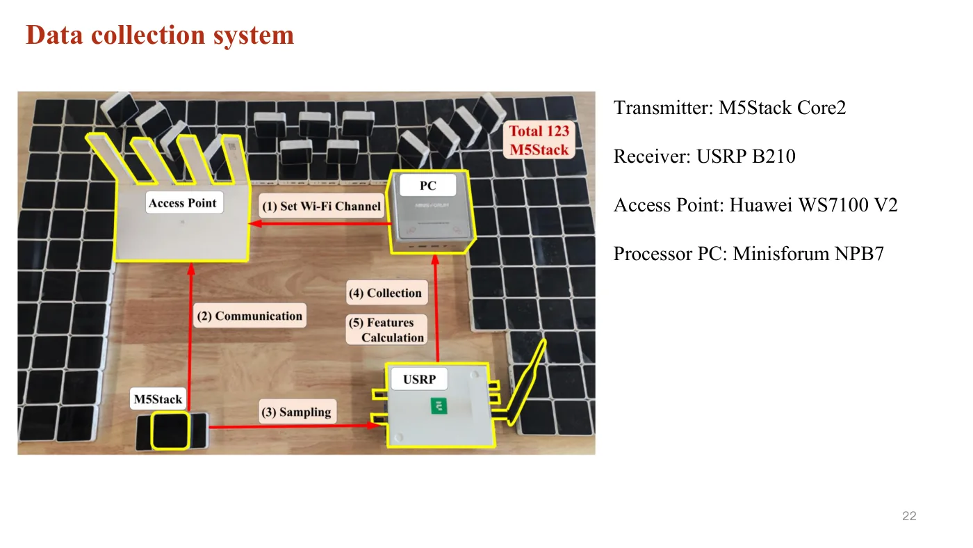
Follow one signal from the M5Stack transmitter to a saved record.
Follow the numbered setup steps
- Set the Wi-Fi channel.
- The M5Stack communicates with the access point.
- The USRP B210 samples the received signal.
- The computer collects the records.
- The processing workflow calculates RF features.
The instructor demonstrates this setup. You will use prepared records in the three labs.
View data acquisition system (opens in a new tab)HANDS-ON LAB · 30 min · SLIDES 24-25
Lab 1: Load and Explore the Dataset
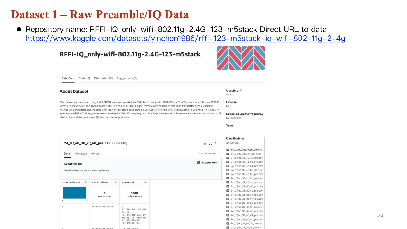
Recognize the two dataset views and the fields the labs will use.
Two dataset views
Raw I/Q: preamble samples and device information.
Feature data: signal-related fields and calculated RF features. Use slide 25 to locate the columns discussed by the instructor.
The two dataset views and the names of the device label, sample, and feature columns.
Follow along
Open the two dataset pages
Open the two dataset links above. Each dataset holds 123 files, one file per device, and each file holds 1000 records. The raw I/Q dataset keeps the device label, the MAC address, and the preamble samples. The feature dataset keeps the same records with the calculated RF features added.
Slide 24 shows the raw I/Q page and slide 25 shows the feature page. Kaggle offers a download button on both pages. The notebook used in the labs, RFF_Data_Calculate, already has both datasets attached, so no download is needed here.
Check: You can say which dataset holds the raw samples and which one holds the calculated features.
Read the columns in the preview table
Each dataset page shows a preview table of one file. Slide 25 lists the columns the instructor will use.
Every file of the raw I/Q dataset holds 3 columns and every file of the feature dataset holds 23. The figure shown on each page, 369 for the raw I/Q dataset and 2829 for the feature dataset, counts the columns of all 123 files.
Find the device label column, the MAC column, the sample column, and the feature columns the labs will use. A sample column holds an array of numbers written as text inside one cell.
Check: You can name the device label column, the sample column, and two feature columns.
Dataset settings and scope
The tutorial uses SMoRFFI as its main case study.
| Property | SMoRFFI Setting |
|---|---|
| Signal type | 2.4 GHz Wi-Fi, IEEE 802.11g |
| Device scale | 123 same-model commercial IoT devices |
| Transmitter platform | M5Stack Core2 |
| Receiver | USRP B210 |
| AP | Huawei WS7100 V2 |
| Capture software | GNU Radio with modified IEEE 802.11 a/g/p receiver components |
| Collection size | 1000 frames per transmitter |
| Raw data | 35.42 million raw I/Q preamble samples |
| Feature data | 1.85 million extracted RF features |
| Sampling rate | 20 MS/s |
| Channel and bandwidth | Wi-Fi Channel 6, 20 MHz bandwidth |
| Environment | Controlled indoor office, static short-distance setup |
| Baseline | Random Forest classifier |
| Reported baseline accuracy | 88.6 percent with Kalman filtering in 5-fold evaluation |
Data Files
SMoRFFI provides two dataset views.
| Dataset View | Contents | Tutorial Use |
|---|---|---|
| Raw I/Q dataset | Device label, MAC address, and preamble samples | Signal inspection and acquisition-to-record mapping |
| Feature dataset | Device labels, MAC addresses, preamble fields, LTS samples, CFO features, phase error, magnitude error, I/Q gain imbalance, and fractal dimension | Feature visualization, baseline training, and evaluation |
Feature Groups
The feature notebook focuses on features that are commonly used in physical-layer identification:
- Frequency-related features: coarse CFO, fine CFO, and combined CFO;
- Constellation-related features: phase error and magnitude error;
- I/Q impairment features: I/Q gain imbalance;
- Shape and complexity features: fractal dimension of processed long training sequences.
The SMoRFFI baseline analysis reports that frequency-related features contribute strongly to Random Forest identification, with CFO, coarse CFO, and fine CFO ranked as the top three features by importance.
Dataset Scope
SMoRFFI is designed for controlled benchmarking of device-feature-based RF fingerprinting in an indoor, static, short-distance, high-SNR setting. Results from this dataset should be reported with that scope. Cross-environment deployment, long-term temporal robustness, and mobile-channel robustness require additional evaluation data.
HANDS-ON LAB · 30 min · SLIDES 27-30
Lab 2: Construct and Visualize RF Features
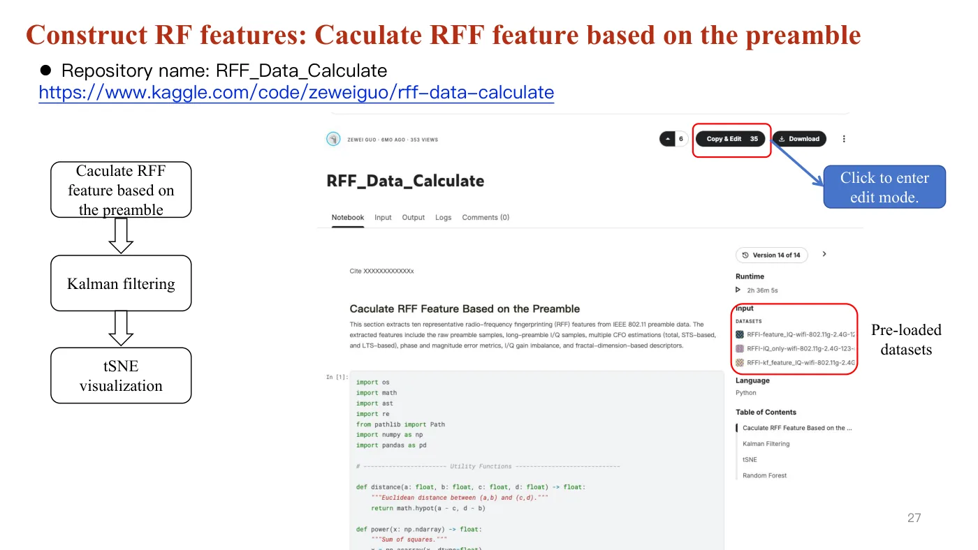
Calculate RF features, apply Kalman filtering, and inspect the t-SNE plots.
Use the notebook shown in the slides
Open RFF_Data_Calculate. Slide 27 shows the notebook entry and attached datasets. Slide 28 shows the cells to run. Slide 29 provides the visual reference.
Open RFF_Data_Calculate (opens in a new tab)Feature calculation → Kalman filtering → t-SNE visualization.
Follow along
Open the editable notebook
Use the notebook link above. Create an editable copy using the copy/edit control. Keep the datasets attached and use the same notebook session for the following steps.
Check: The first code cell is available to run.
Calculate features from the preamble
Find the feature-calculation section shown on slides 27-28. Run the imports and helper definitions first, then the calculation cell. Wait for each cell to finish before continuing.
Read the input and output paths in the cell. Note where the calculated feature records are stored.
Check: The calculation finishes without an error, and the output contains calculated feature values.
Run Kalman filtering
Continue to the Kalman Filtering section shown on slide 30. Read which feature columns it processes, then run the cell. Keep the unfiltered output available for comparison.
Check: Both the unfiltered and filtered feature data are available to the visualization step.
Run t-SNE and compare the plots
Run the t-SNE visualization section. Compare the plots for the same device selection before and after filtering, using slide 29 as the reference.
Observe clusters, overlap, and spread. Exact point locations can vary with the selected records and t-SNE settings. Use Lab 3 to check the corresponding identification results.
Check: You can display both plots and describe one visible difference.
If a later cell fails
First check that the preceding cell completed. For missing variables, run the earlier definition cells. For missing files, compare the output path from feature calculation with the input path used by filtering or visualization. Keep the device selection consistent between the plots.
HANDS-ON LAB · 30 min · SLIDES 32-36
Lab 3: Build and Evaluate the Baseline
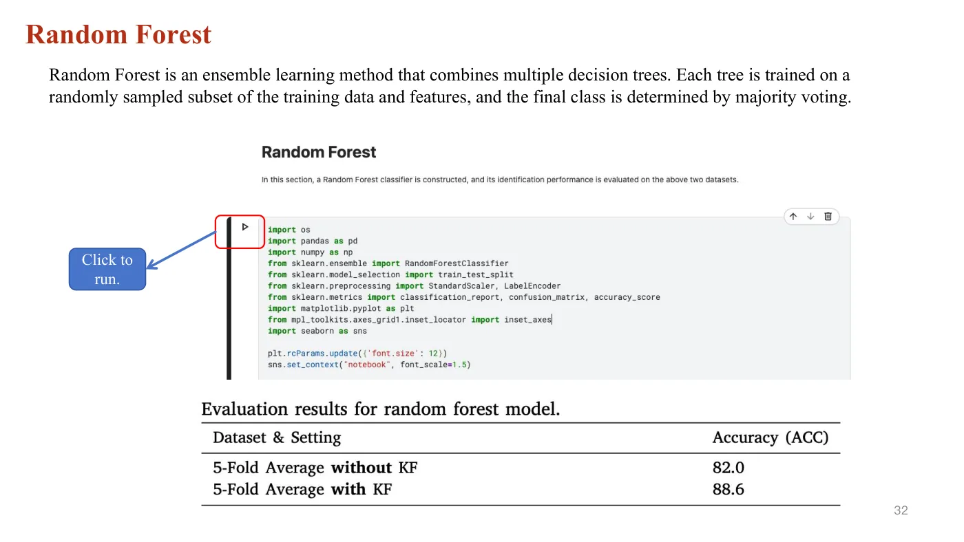
Run the baseline and read the results produced by the experiment.
From features to device predictions
Continue to the Random Forest section of the notebook. Read the result table, feature-importance output, and confusion matrix alongside slides 32-36.
Continue in the notebook (opens in a new tab)Your accuracy result, the most important features, and an explanation of at least one pattern in the confusion matrix.
Follow along
Run Random Forest
Continue to the Random Forest cell shown on slide 32. Identify the selected feature columns, device labels, and evaluation setting in the code. Run the cell after the feature-processing cells have finished.
Check: The cell produces predictions and an accuracy result.
Read the accuracy results
Compare the unfiltered and filtered results. The slide screenshots report the following reference values.
Reference: slide 32. These are the reported slide results. A different device subset, split, preprocessing configuration, or software version can produce different results.
Check: You have recorded your data selection, evaluation setting, and accuracy.
Inspect feature behavior and importance
Read the feature traces on slide 33 and the importance table on slide 34. Locate CFO, coarse CFO, and fine CFO in the table. Compare the notebook output with this ranking.
Check: You can identify the highest-ranked features in your result.
Read the confusion matrix
Use slide 35 as a guide: the vertical axis is the true device label and the horizontal axis is the predicted label. Diagonal entries correspond to correct predictions. Off-diagonal entries show confused device pairs.
Inspect the displayed matrix and select a visible off-diagonal entry. Identify the true and predicted device labels.
Check: You can explain one correct prediction pattern and one device confusion.
Compare feature groups
Read slide 36 from left to right. Use slide 34 to map f1 through f15 to feature names. Compare the accuracy bars as more features are included, and compare the filtered and unfiltered cases.
Check: You can relate a feature-group result to the features used in that experiment.
GUIDED SESSION · 20 min · SLIDES 38-41
Summary and Open Discussion
Review the experiment you have completed.
- Loaded Wi-Fi records and identified their fields.
- Calculated and visualized RF features.
- Trained a baseline and inspected its results.
Discuss the results
Which features contributed most? Which devices were confused? What would you check before using the workflow in another environment?
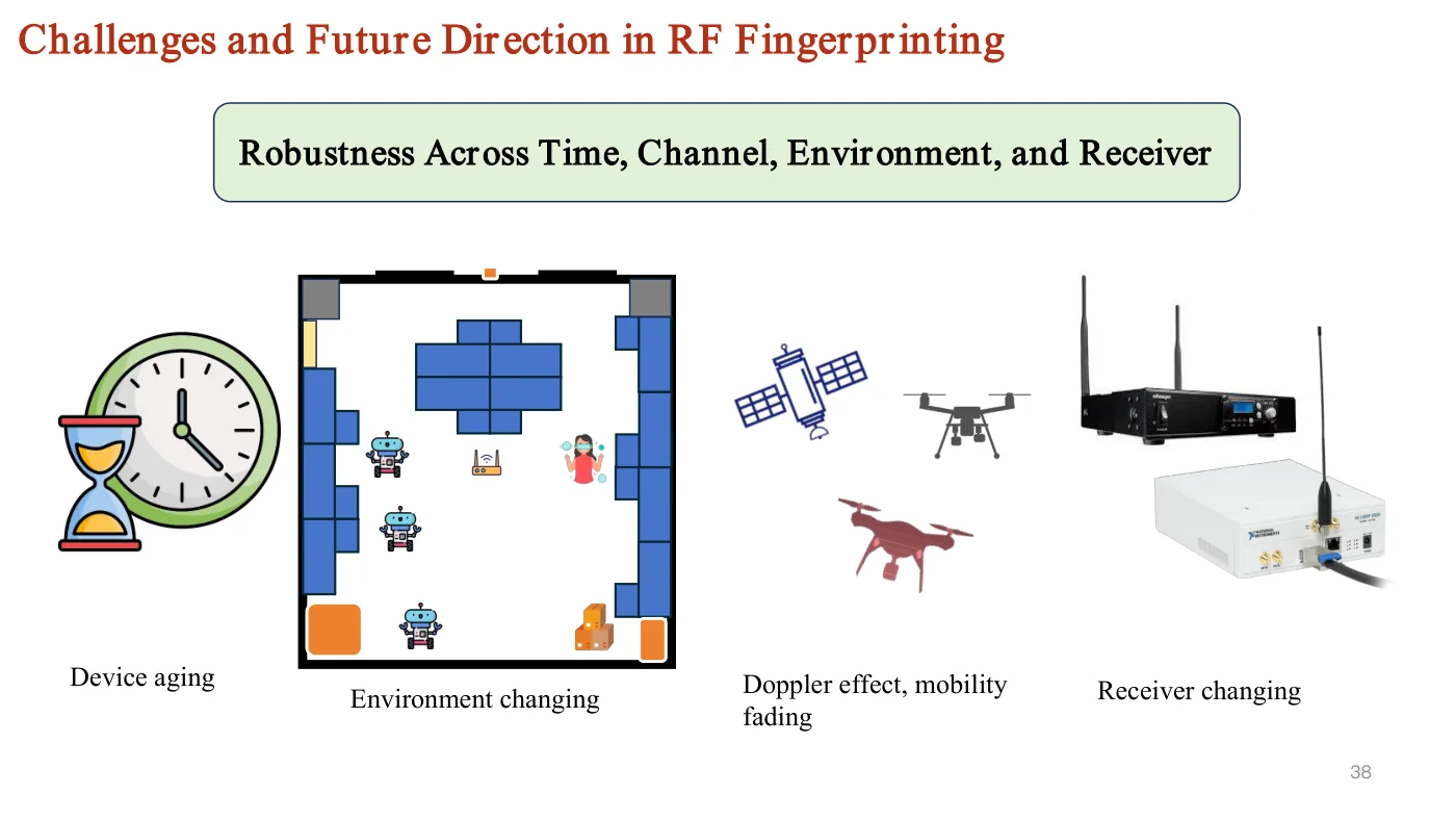
Slides 38-40 introduce feature robustness, device scale, reproducibility, and attacks. Use these topics for the closing discussion.
Reproducibility checklist
Use this checklist when running or adapting the notebooks.
| Item | What to Record |
|---|---|
| Data version | Dataset name, download date, subset name, and file count |
| Device labels | Number of devices, label field, and sample count per device |
| Feature set | Included features and any filtering or smoothing |
| Split design | Train-test split, cross-validation setting, random seed, and device/sample grouping |
| Model | Algorithm, hyperparameters, software versions |
| Metrics | Accuracy, recall, F1-score, confusion matrix, and per-device results when available |
| Reference check | Matching checkpoint outputs or documented differences |
| Scope | Environment, channel setting, hardware setting, and limitations |
COURSE INFORMATION
Tutorial information
Responsible use
The tutorial uses controlled laboratory device data. The tutorial dataset does not include human-subject data, personal identity information, user behavior logs, or application-layer communication content. Device labels correspond to laboratory-owned IoT devices.
During the tutorial, no personal wireless devices will be recorded. Any hardware interaction uses organizer-provided equipment.
Responsible RFF research requires controlled data collection, compliance with local radio regulations, careful handling of identity-sensitive deployments, and clear separation between laboratory benchmarks and real-world tracking scenarios.
Organizers, contact, and citation
- Jinxiao Zhu, Tokyo Denki University, Japan
- Zhen Jia, Reitaku University, Japan
- Wenhao Huang, Keio University, Japan
- Zewei Guo, Future University Hakodate, Japan
- Yin Chen, Reitaku University, Japan
Contact
For questions about the tutorial, please contact:
Zhen Jia Reitaku University, Japan jiazhen0628@outlook.com
Citation
If you use the dataset or reproduce the benchmark, please cite the SMoRFFI article:
Zewei Guo, Zhen Jia, Jinxiao Zhu, Wenhao Huang, and Yin Chen. 2026. SMoRFFI: A large-scale same-model 2.4 GHz Wi-Fi dataset and reproducible framework for RF fingerprinting. Computer Networks, 282, 112309. DOI: 10.1016/j.comnet.2026.112309.
Tutorial paper: Zhen Jia, Jinxiao Zhu, Wenhao Huang, Zewei Guo, and Yin Chen. 2026. Tutorial: Building Reproducible Wi-Fi RF Fingerprinting Pipelines: Signal Collection, Datasets, and Evaluation. UbiComp Companion ’26. doi:10.1145/3798063.3836754.
ACKNOWLEDGMENT
Acknowledgment
This work was partly supported by JST Moonshot R&D Grant Number JPMJMS2215, JSPS KAKENHI Grant Number JP24K07482, and the Research Promotion Program for Security Technology (Grant Number JPJ004596) of Acquisition, Technology & Logistics Agency in JAPAN.
Back to the top ↑